
OCR is short for Optical Character Recognition, this is the technology used to identify the text from images. As is with any other computer vision related project, the first thing to carry out OCR is that you need a clean image of the text document. The lighting conditions and resolution of the text in the image play a big role in carrying out OCR successfully. Once you have that you need break down the complete process into multiple parts and then solve them independently. I have described below some steps that need to be done for successfully carrying out OCR
Steps to be done for OCR
- Finding Region of Interest (ROI)
- Cleanup / rotate / transform the located document
- Segmentation of relevant area of image
- Carry out OCR
Discussing all the parts is going to be a big topic in itself, so in this blog post we shall mainly focus on point #1
Finding Region of Interest (ROI)
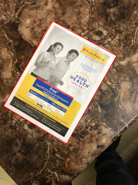
Need to identify and locate the document in the image this region is called ROI. This can be really tricky part and the process to extract ROI (region of interest) will vary a lot based on the type of image, document background, lighting conditions etc. For example look at the below images:
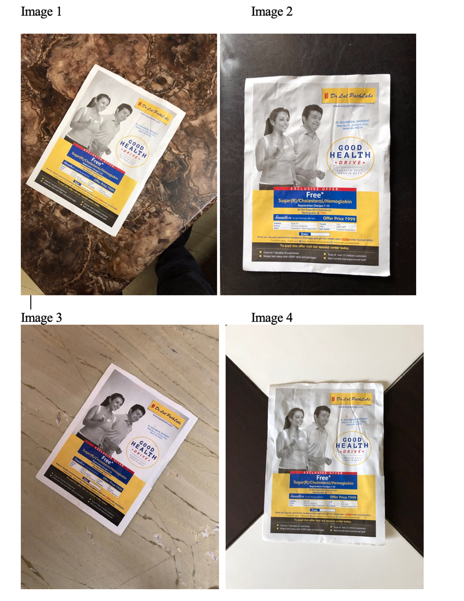
We shall be using the same document with 4 different backgrounds to demonstrate how it can be challenging to separate out our region of interest from the background.
Some points to note:
- The document is rectangular in shape
- It has multiple rectangles within the document that can be confused with the document itself
- The document is not always in horizontal position
- The document has white border that can be used to separate it out from the background
We would need to separate out the image from the background, and image histogram is a very handy tool to analyze the images and related pixel intensities. Here is the histogram for all 4 images.
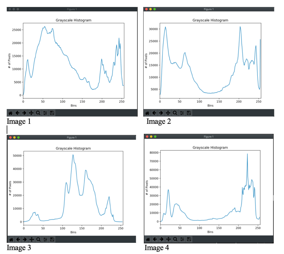
As we can clearly see from histogram for image 2 and 4 that there are 2 peaks clearly separated however on image 1 and 3 there is no such very clear demarcation.
So we setup simple algorithm:
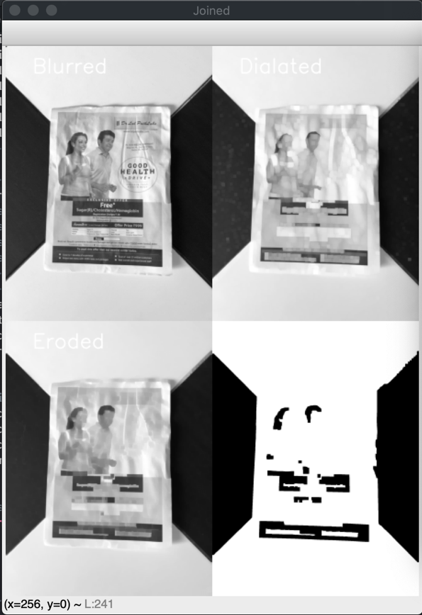
- Blur the image using Gaussianblur, 7X7 kernel to blur the image details that we are not interested at this point.
- Then we run a carry out multiple dilations and erosions to get rid of the details in the document, which anyways we are not interested in at this point.
- And finally we run (normal, OTSU’s and Adaptive) threshold to see if we can get the rectangle of the document (ROI) clearly.
- Then we try to find contours on the thresholded image. When looking for contours we run it with parameter RETR_EXTERNAL so that only external contours are returned.
- Then using approxPolyDP we try and see if we can get any contour with just 4 corners.
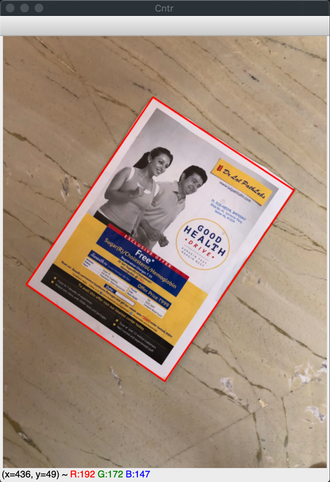
- If we get an contour with 4 corners we draw the contour
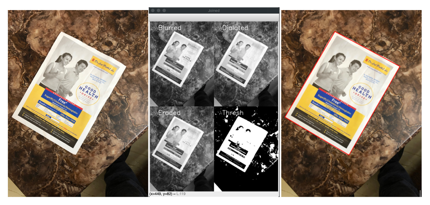
Starting with the first image
Voila! We can see that our ROI has been correctly identified, as can be seen in the image above. We did not have to do anything much in this case. Similarly when we run the same code with image #2, it works like a charm. Since in both the cases the background was clearly and easily distinguishable from the text document.
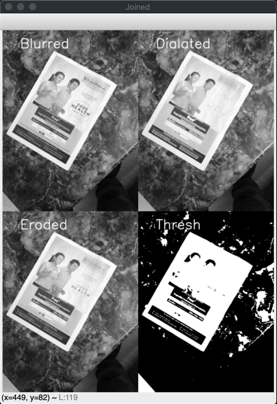
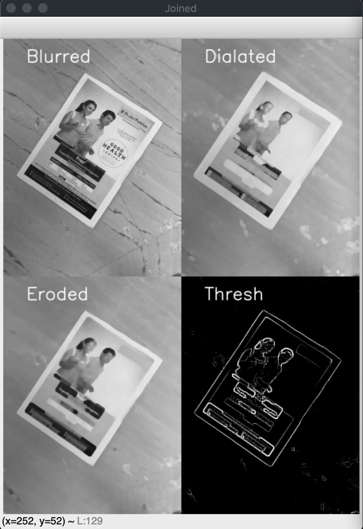
Going to the image # 3, it seems a little bit difficult since the color difference between background and document is not very significant. When we run our current algorithm (which worked easily on image #1 and 2), it gives below results
Which does not look good. So it seems OTSU’s threshold that determine one unique value for thresholding is not a good way to go about this image. Since the background and foreground are similar, it is going to be difficult to separate them out with just one value.
Lets try adaptive threshold on this one and see how it works
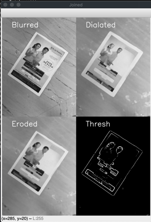
It still does not work but looks quite encouraging. We can see clear boundary of edges. So let’s try to make the edges sharper and see if that helps.
This helps us locate our document.
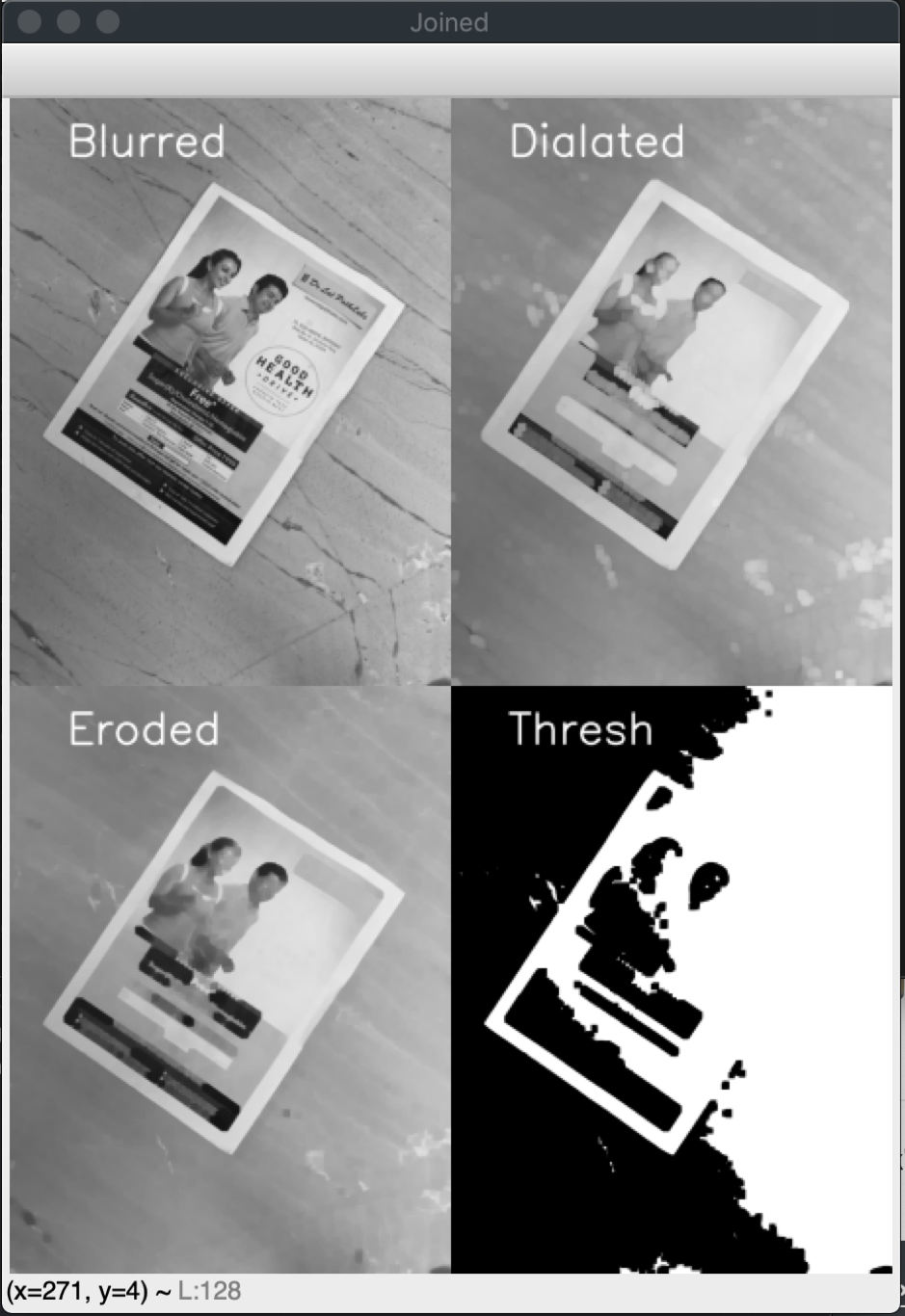
Let’s look at image #4, this seems like a really tricky image to get our ROI. As we can see the background has complete dark as well as light colors. But starting with OTSU’s threshold, let’s see what we get.
This looks exactly as we thought. The document boundaries merge with the background making it very difficult for us to get ROI. Let’s try next with Adaptive threshold.
As we can see above, it does give us some boundaries, however, it is still very difficult to segregate our ROI. Let’s look at image histogram to see if we can get some additional information.
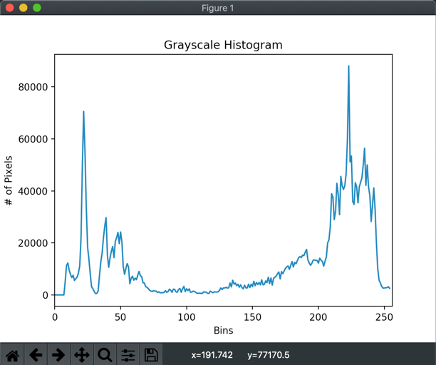
The histogram shows 2 very distinct peaks, however we know that peak between 200 and 250 has background as well as the image ROI that we are interested in. We can probably dig deeper and still try to find the ROI on this image, but this is going to be very difficult if not impossible. But here I’d like to reiterate that we need to keep background and document image separate as much as possible so that getting ROI is not as complex.
Let’s dive into the code on how we are doing things:
You can download the code and all images at OCR Preprocessing- ROI so you can try the same and follow along with the blog.
#working with openCV version 4.1.2
import cv2
#pip install imutils
import imutils
import numpy as np
from matplotlib import pyplot as plt
The line 1 to 6 are simply importing the required packages. Imutils is a package that many helper functions for images by Adrian. We are importing pyplot as we will need to plot image Histogram.
def locateRegion(img):
    #gray
    gray = cv2.cvtColor(img,cv2.COLOR_BGR2GRAY)

    #At times it is beneficial to break the image into individual components
    # and then use the same to see if we can get the rect.
    #lab=cv2.cvtColor(img,cv2.cv2.COLOR_BGR2Lab)
    #b,g,r = cv2.split(lab)
    #gray = b
On line 10 we define a function locateRegion. In this function we shall try to pre-process the image such that it becomes easy to find the document part in the given image (ROI). We start with converting the image into gray scale image on line 12. Line number 16 to 18 are commented, however are very useful in some cases (the approach works particularly well in case there is less difference between background and ROI for example image 3 in our case)
    #blurr
    blurred = cv2.GaussianBlur(gray, (7, 7), 0)
    #dialate
    dialated = cv2.dilate(blurred, None, iterations=10)
    #erode
    eroded = cv2.erode(dialated, None, iterations=10)

    #sharpening kernal
    kernel = np.array([[-1,-1,-1], [-1,9,-1], [-1,-1,-1]])
    sharp = cv2.filter2D(eroded, -1, kernel)
On line 21 we are initially blurring the image initially using a 7X7 kernel and then carry out morphological operations of dilation and erosion on lines 23 and 25 to reduce the details in the image so that we can easily get the boundaries of document. Finally on line 28 we define a sharpening kernel and then convolve the same on line 29 to increase the sharpness of lines in the image obtained after erosion. You can read up a good description of how convolutions work with images here
    hist, bins = np.histogram(eroded, np.array(range(0, 256)))
    # enable below line if you want a normalised Histogram
    #hist /= hist.sum()
    plt.figure()
    plt.title("Grayscale Histogram")
    plt.xlabel("Bins")
    plt.ylabel("# of Pixels")
    plt.plot(hist)
    plt.xlim([0, 256])
On line 31 we generate histogram for the image and visualize the same. You will notice that we have used bin range from 0 to 256 instead of 0 to 255. Since the way np.histogram works, the last bin (if we had used end limit as 255) would be 254 and 255 which would include pixel values for both 254 and 255, however we do not want that, we want values separately for 254 and 255 hence we use end limit as 256 (1 more than actual values possible)
    #try for image 4
    #thresh = cv2.threshold(sharp, 206, 255, cv2.THRESH_BINARY )[1]
    # OTSU's threshold for image 1 and 2
    thresh = cv2.threshold(eroded, 0, 255, cv2.THRESH_BINARY | cv2.THRESH_OTSU)[1]
    # adaptive threshold for image 3
    #thresh = cv2.adaptiveThreshold(sharp, 255,cv2.ADAPTIVE_THRESH_MEAN_C, cv2.THRESH_BINARY_INV, 31, 17)
Lines between 42 and 47 list down multiple ways we can threshold the image.
Thresholding is operation where we convert the image into a binary image. Binary image is which has only 2 intensities 0 or 255. Basically, line number 43 (commented) uses simple thresholding. Where we pass the image as the first parameter on which we need to apply threshold. Second parameter is the threshold value which will be used to convert the image into binary. The pixel intensities which are less than threshold are converted to min value (0) and then ones that are more than the threshold are converted to max value (provided as 3rd argument)
Then on line 45 we use Otsu’s threshold. Basically Otsu’s threshold is a way to calculate the threshold value automatically based on image pixel intensities. Otsu’s method works well when we are working with bimodal images (bimodal image is one that has 2 clear separated out peaks in pixel intensities). It works well to find the value of threshold which lies between the 2 peaks of pixel intensities. You would notice that we are calling the same function as normal threshold. The first parameter is the image we want to threshold, second parameter is ignored in this case since Otsu’s method calculates the threshold value on its own and discards the value we provide, third param is the max pixel intensity that we want to use. Notice the last param where we pass the param indicating that we want to use Otsu’s threshold.
On line 47 we have the adaptive threshold. Basically the Otsu’s threshold finds the single best threshold value for the image, however at times the illumination of image is such that we may need different threshold value for different regions. That’s where we use adaptive threshold. We pass in the image to be threshold as the first parameter, second param is the max pixel intensity, then we pass the parameter that is used to calculate the mean for the given region. The last 2 parameters specify how many pixels (31 in our case) need to be examined in the neighborhood and what constant (17) needs to be subtracted from the mean value. These are the 2 variables that you can play with to see which value works well for you.
You can read more about thresholding at https://docs.opencv.org/master/d7/d4d/tutorial_py_thresholding.html
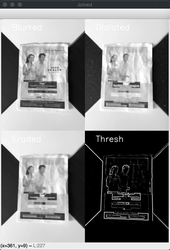
    # add text on top of all images so we can easily visualise all of them
    blurred = putText(blurred, "Blurred")
    dialated = putText(dialated, "Dialated")
    eroded = putText(eroded, "Eroded")
    thresh = putText(thresh, "Thresh")
    #Join images to show all, need to show images in 2X2 matrix
    JoinedImage1 = np.concatenate((blurred, dialated), axis = 1)
    JoinedImage2 = np.concatenate((eroded, thresh ), axis = 1)
    JoinedImage = np.concatenate((JoinedImage1, JoinedImage2))
    cv2.imshow("Joined", imutils.resize(JoinedImage, height = imgSize))

    # show the plot using matplot lib
    plt.show()

    return thresh
Now we want to visualize all the images and how that look after each step, so we have created a grid of 2X2 and joined our images together to display them as one image. This could have been accomplished via matplotlib as well but at times we find this useful.
On line 62 we display the plot we have generated. And finally we return the thresholded image from the function on line 64
#Add text on top of images and return the same image back
def putText(img, text):
    return cv2.putText(img, text, (200 ,200), cv2.FONT_HERSHEY_SIMPLEX, 5, (255,255,255), 10)
On line 66 and 68 we have a small utility function that adds the text on top of image provided and returns the same.
def findContourAndAddLayer(thresholdedImg, OriginalImg):
    foundCntrs = False
    #we shall calculate solidity to see if we are looking at right 4 point contours
    solidity = 0
    ratio = 0
    screenCnt = None
    OriginalImg = OriginalImg.copy()
    output = OriginalImg.copy()
    thresholdedImg = thresholdedImg.copy()
Then we simply initiate the function that will find the ROI from the thresholded image. On lines 72 through 80 we simply initialize the variables that we will need in this function.
    cnts = cv2.findContours(thresholdedImg, cv2.RETR_EXTERNAL, cv2.CHAIN_APPROX_SIMPLE)
    cnts = imutils.grab_contours(cnts)
    cnts = sorted(cnts, key=cv2.contourArea, reverse=True)[:5]
On line 82 we try to find the contours in the thresholded image. Notice that findContours function modifies the image that it passed to it. Hence we have made a deep copy of image that was passed to the function on line 80. We are only interested in external contours hence we pass cv2.RETR_EXTERNAL and we have used cv2.CHAIN_APPROX_SIMPLE which optimizes the contour detection. You can read more about these variables at https://docs.opencv.org/2.4/modules/imgproc/doc/structural_analysis_and_shape_descriptors.html#findcontours
The function returns tuple of all the contours it has found. Since OpenCV returns different format for tuple in different versions hence we are using utility function from imutils that provides contours in version independent way. On line 85 we sort the contours we got based on their area and return only top 5. Though we may be interested only in the biggest contour however we shall analyze top 5.
    for (i, c) in enumerate(cnts):
        peri = cv2.arcLength(c, True)
        approx = cv2.approxPolyDP(c, 0.02 * peri, True)
        if len(approx) == 4:
            screenCnt = approx
            #get min rect that can bound the contour we have found
            rect = cv2.minAreaRect(c)
            box = cv2.boxPoints(rect)
            #calculate the area of the bounding rectangle
            rectArea = cv2.contourArea(box)
            #calculate area of the contour
            shapeArea = cv2.contourArea(c)
            #calculate colidity, which needs to be > 0.75 for it to be the shape we are looking for
            solidity = shapeArea / rectArea
            totalImageArea = OriginalImg.shape[0] * OriginalImg.shape[1]
            ratio = shapeArea / totalImageArea
            # solidity should be very high since our ROI is rectangular in itself
            # ratio represents the ratio of identified rect area Vs total image area
            # Remember area ratio varies as square of the perimeter so 0.2 is generally
            # big enough
            if solidity > 0.80 and ratio > 0.1:
                foundCntrs = True
                cv2.drawContours(output, [screenCnt], -1, (0, 0, 255), 5)

            break
The on line 85 we loop through the contours thus obtained. We calculate the length of the contour on line 86 using OpenCV function. The second parameter is to indicate that we want to calculate perimeter of closed contour.
Line number 87 is a very interesting and useful function call, approxPolyDP. This function can be used to approximate a curve with lesser points. An important parameter for this approximation is second parameter which is epsilon which is “Parameter specifying the approximation accuracy. This is the maximum distance between the original curve and its approximation.” The last parameter for the call is whether we are looking for a closed curve.
Since this is a very important function, it’s better to understand this in depth. This function works based on Ramer–Douglas–Peucker algorithm
Below image explains how the algo works and reduces the number of points based on epsilon.

You can read more about this function at https://docs.opencv.org/2.4/modules/imgproc/doc/structural_analysis_and_shape_descriptors.html
Also, there is a very interesting visual tool to understand the working of the algorithm here
The function returns the approx. number of points that would be used to represent the curve and since in our case we are looking for a rectangle, we check if the number of points returned are 4 in the next line (88). If the number of points is indeed 4 then we do a few more checks to ensure that we are looking at a big enough rectangle that we may be interested in.
For example we calculate solidity of the curve thus obtained. If the ratio of minimum bounding rect and curve area is high then we know that it is indeed a rectangle that we are looking at. Then we also compare that the total area of the curve Vs total image area is within a threshold so we are looking at big enough rectangle.
Once these checks are done successfully we assume that we have found the correct rectangle. We draw the contour on line # 107 and then return the image
#set display image size
imgSize = 600
imagePath = "./im3.jpg"
img = cv2.imread(imagePath)
#preprocess the image to highlight the location where we want to find the document
thresh = locateRegion(img)
#locate contours and find and display the rect as it is found
(cntr, found, screenCnt) = findContourAndAddLayer(thresh, img)

# If the ROI has been found display it on screen
if (found):
    cv2.imshow("Cntr", imutils.resize(cntr, height = imgSize))
cv2.waitKey(0)
On these lines we just invoke the functions that we have created with the images. On line 121 we read the image and then pass it onto functions to find ROI.
We have discussed many useful functions in this blog. Since you will be using these quite a lot if you are going to be doing something similar so it would be useful if you understand this in detail. Also one thing to note is, one simple algorithm with same threshold values will not work for all images. Hence when processing files for OCR you need to device a strategy where you can try different ways to identify ROI.
You can download the code and all images at OCR Preprocessing- ROI
References:
All the references for this blog are added inline so that they are more accessible.