
There is so much work going on #MachineLearning and #DeepLearning space. The basis of most of that is the artificial neural networks. I assume that you understand ANN well and are now trying to implement the same. If you do not understand it yet, then consider going through this blog. In this Blog I am going to implement neural network in python, just to understand their inner workings. This will be a good primer to understanding how Keras / tensorflow or pyTorch allow us to code at much higher level abstracting the internal details and make our lives as deep learning professionals much easier.
The code for the below steps can be downloaded from Neural Network code
I am going implement a neural network (nn) class in python which shall incorporate training the weights and then use the class for predictions. We shall run MNIST (sample dataset) [reference] and the downloaded code would also work on MNIST (original dataset) [reference].
Step 1: We shall create a class named neuralnet and implement the reusable neural network logic in neuralnet.py
class neuralnet:
#class level variables
#ctor
	def __init__(self, architecture ):
		self.architecture = architecture
		self.archiLen = np.size(architecture)
Line 1 simply creates a class named neuralnet and then on line 4 onwards we implement the constructor. The constructor takes in a variables which is the architecture of neural network. For example if you want to create a simple 3 layer nn with 1 input layer (with 2 inputs), 1 hidden layer (with 3 nodes) and 1 output layer (2 class classifier) then you will pass in an array [2,3,1] for architecture (will use [2,3,1] nn architecture as example in the rest of the article to explain concepts). On line 5 and 6, we use the input variable to initialize the class level variable and set the length of architecture in archiLen variable.
		self.W = []
		#initialise weights based on architecture
		#if there are n layers on the nn, then we will have n - 1 weights
		#also last layer weights are special case
		for i in range(0, self.archiLen - 1):
			if i < self.archiLen - 2 :
				self.W.append(self.initialiseWeights(self.architecture[i] + 1 ,self.architecture[i+1] + 1))
			elif i == self.archiLen - 2 :
				#output layer is a special case, it has no bias
				self.W.append(self.initialiseWeights(self.architecture[i] + 1, self.architecture[i + 1]))
In the above mentioned architecture [2,3,1], we will have 2 sets of weights, one for calculating activations from input layers to hidden layer and other from hidden layer to output.
*I assume you understand the basics of neural networks and how it works, if not Andrew Ng’s lecture on coursera ML course is must watch
On line 8 we have declared our weights (W) and then we are using loop to initialize the same. The important point to note here (in the loop) is, we need to handle the output layer differently from each of the other layers. All other layers (including input layer), we will need to add a node for bias which is not the case for output layer. The ‘if’ condition checks for the same. As the weights are initialized they are appended to the class level weights matrix.
	def initialiseWeights(self, currentLayer, nextLayer):
		w = np.random.randn( currentLayer , nextLayer)
		#w = (np.random.randn( currentLayer , nextLayer) * np.sqrt(1/currentLayer))
		return w
On line number 19 to 22 we define a function that initialises the weights matrix with the random set of initial weights. We have used standard normal random values for weights initialisation (however, it is advised to use weights inversely proportional to the square root of the number of neurons in the current layer [Reference 2], as done on line number 21 commented code. My observation has been standard normal random number tends to converge faster than the other.
        def sigmoidActivation(self, z):
		g = 1.0 / (1 + np.exp(-z))
		return g

	#assuming we are getting activations and since they are already
	#applied with sigmoid so no need to apply sigmoid again
	#Formula for derivative sigmoidAct(z) * (1 - sigmoidAct(z))
	def sigmoidDerivative(self, act):
		return act * (1 - act)

	def calculateZ(self, X, w):
		return X.dot(w)
Then between lines 24 and 35 we define some standard functions for calculating Sigmoid Activation, its derivative etc.
	def calculateActivation (self, x ) :
		activation = []
		activation.append(x)
		for j in range (0,self.archiLen-1):
			activation.append(self.sigmoidActivation( self.calculateZ(activation[-1], self.W[j]) ))
		return activation
Between line 39 and 44, we define the function that calculates activation for all the layers in our neural network. The function takes input vector as an input, appends the same as initial activation for the input layer, and then calculates activation for the next layer based on this and appends the same to activation variable. By the end of the loop, we have activations calculated for all the layers of neural network. The activation for output layer is same as the output of the network.
	def train(self, X, Y, epochs = 100, alpha = 0.01):
		epochCost = []
		#Add bias to inputs
		bias = np.ones((len(X),1))
		XwithBias = np.hstack((X,bias))
On line 48, we define the train function that is used for training the network. It takes input vector X, output vector Y, epochs (number of iterations we want to train the network for) and alpha (learning rate) as inputs. We have assigned default values for epochs and alpha. Then we add the bias to the input vector.
		for i in range (0, epochs):
			cost = 0
			for (x, y ) in zip (XwithBias, Y):
				act = self.calculateActivation (x)
				error =  self.backprop (act, y, alpha)
There is a lot happening between lines 54 and 58.
We start with the loop which runs for number of epochs as provided in input, then on line 55 initialize the cost of the network for the current epoch with 0. On line 56, we iterate on the input vector, and run through forward propagation to calculate activation on line number 57. We then use the output (activations) from forward propagation to run the back propagation on line 58. Back propagation is the process where weights are optimized based on the error calculated from forward propagation.
			cost += np.sum(np.square(error[-1]))
			#Calculate Cost for this iteration
			cost = (1/Y.shape[0] ) * cost
			epochCost.append(cost)
On line 59 we accumulate the error of the current epoch based on the error and then on line 61 we compute mean squared cost for the current epoch.
	def backprop (self, act, Y, alpha):
		#calculate the output error by simply finding difference between
		#output later activation and correct labels
		error = act[-1] - Y
		Delta = [error]
On line 68 we have defined back propagation for our neural network implementation. Then we calculate the error by computing the difference between the output layer activation and the actual output on line 71. This error value is stored as initial delta (on line 72) for the output later which will be propagated backwards to compute optimized weights.
		for i in range (0,self.archiLen-2):
			wT = np.transpose(self.W[self.archiLen - i - 2])
			delta = ((Delta[-1]).dot(wT))
			delta = delta * self.sigmoidDerivative(act[self.archiLen - i - 2])
			Delta.append(delta)
Between lines 75 and 79 we are back propagating the delta for the output layer through the network to compute delta for each of the layers. Note: delta is not computed for the input layers (notice archiLen-2), hence, in the loop, we only need to calculate delta for 1 hidden layer in our example architecture [2,3,1].
		for i in range (0, self.archiLen - 1):
			self.W[i] += -1 * alpha * (np.transpose(np.atleast_2d(act[i]) ).dot(np.atleast_2d(Delta[i])))
Based on the delta values calculated for each of the nodes in the hidden layer, we need to now calculate the updates in the weights. This is the part where actual learning in the network is taking place. On line 87 we run the loop for all the layers in the network, and then on line number 88 we compute the change in weights using learning rate, activations from forward propagation and delta computed in the previous steps. The change in the weight is then added to the respective weights to arrive at the updated weights for the layer.
	def predict (self, X, Y ) :
		act = []
		#append Bias term
		bias = np.ones((len(X),1))
		XwithBias = np.hstack((X,bias))
Finally we need to implement the prediction function, that will take input as test inputs (X) and test output(Y). We need to add bias to the inputs.
		for (x, y ) in zip (XwithBias, Y):
			act.append(x)
			for j in range (0,self.archiLen-1):
				act.append(self.sigmoidActivation( self.calculateZ(act[-1], self.W[j]) ))
			predictions.append(act[-1])
		return predictions
Then on line 101 we run the loop on the input values. On line 103 and 104, we propagate the input values through our network and calculate the activation for the output layer. We are using the weights that our network learned during the training process, so if our network has learned the right weights it must do the right predictions
On lines 105 and 106 we accumulate the predictions for all values of input X and Y and return the same.
Step 2: Now we shall use this class created in step 1 above and see if it works with MNIST [Reference] (sample 8X8 dataset) (nn.mnist.py)
import math
import numpy as np
from codedeepai import neuralnet
from sklearn.preprocessing import LabelBinarizer
from sklearn.model_selection import train_test_split
from sklearn.metrics import classification_report
from sklearn import datasets
# Uncomment below to work with original dataset
#from sklearn.datasets import fetch_openml
import matplotlib.pyplot as plt
Lines 1 through 10 Import the required packages, on line 3 we import the class that we just created above. Line number 9 is commented, if you want to work with original MNIST (28X28 dataset, 70,000 sample data) digits then uncomment the same. It is much bigger dataset compared to sample (8X8, ~17000 data points) and would require considerable amount of training time.
print("loading MNIST data...")
digits = datasets.load_digits()
# uncomment this line if you want to use original Mnist dataset
#digits = fetch_openml('mnist_784', version=1, cache=True)
data = digits.data.astype("float")
data = (data - data.min()) / (data.max() - data.min())
print("samples: {}, dim: {}".format(data.shape[0],
	data.shape[1]))
Lines 13 through 19 load the MNIST data and normalize (scaling it between 0 and 1) the input data.
(trainX, testX, trainY, testY) = train_test_split(data,
	digits.target, test_size=0.25)
Then on line 23, using sklearn we split the dataset into test and training set with 25% data for testing.
trainY = LabelBinarizer().fit_transform(trainY)
testY = LabelBinarizer().fit_transform(testY)
Then using sklearn’s LabelBinarizer, we binarize the output vector. Basically with digit classification we are doing a 10 class classification, hence the output vector contains values like 0,8,1 etc. We need to represent it as one hot encoding format.
architecture = [64,16,12,10]
On line 36 we are initializing the network architecture. Since the input images have 8X8 pixels so we are using 64 nodes in the input layer, we are using 2 hidden layers with 16 and 12 nodes. Since this is 10 class classification (digits from 0 to 9) we are using 10 nodes in output layer
nn = neuralnet(architecture)
epoch = 100
alpha = 0.1
cost = nn.train(trainX, trainY, epoch, alpha)
On line 40 we create an object of the neuralnet class and initialize the epoch and alpha (learning rate) variables and then initiate the training of the network based on our variables.
predictions = nn.predict(testX, testY)
predictions = np.asarray(predictions)
predictions = predictions.argmax(axis=1)
correct = testY.argmax(axis=1)
print(classification_report(correct, predictions))
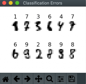
On line 50 we run the predictions on our trained network for the test set. Then use predictions to display classification report (confusion matrix, f1 score etc.) using sklearn. Here is the details of the results obtained
result = np.nonzero(correct - predictions)
#incorrect image index
index = []
for i in np.nditer(result) :
	print ("Actual: {} Predicted: {}".format(correct[i], predictions[i]) )
	index.append( (data == testX[i]).all(axis=1).nonzero()[0][0] )
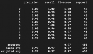
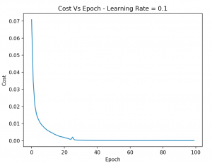
As we were interested to see which numbers were not predicted correctly, below the visualisation of numbers that were predicted incorrectly by our neural network.
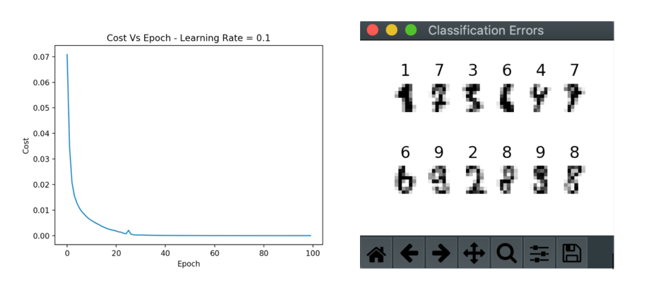
And finally here is the Cost Vs Epoch graph
Add references
Reference 1:
Andrew Ng’s course on Machine learning, run through chapter 8 and 9
Reference 2: Better weight initialization for neural networks
Reference 3: Interesting way to visualise Neural Networks
Download the code and play with it to see how it works Neural Network code
Please feel free to add your questions and comments below